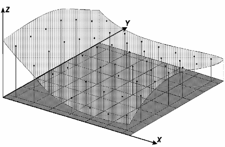
The rectangle or regular grid is a digital model that shape surfaces through rectangle face polyhedron. Vertexes of those polyhedra can be the sampled points in case they have been acquired in same XY locations that define the wanted grid.
The
rectangle grid
generation must be done when a sampled data in the surface is not
obtained with regular spacing. Thus from isoline contained information
or in sampled points it is generated a grid that represent as closest
as possible to the real surface. Initial values to be determined are x
and y coordinate space in a way they can represent close values to the
grid points in big variation regions. At same time, they should reduce
redundancies in almost plane regions.
The grid space,
i.e. x and y
resolution, should be ideally lower or equal to the lower distance
between two samples in different quotas. When generating a very thin
grid (dense), with a very small distance between points, there will be
a bigger amount of information about the analyzed surface, but will
need more time to generate. Otherwise considering big distances among
points, it will be created a thick grid that could lose information.
Therefore, the final grid resolution must have a commitment of data
accuracy and grid generation time.
Once defined the
resolution
and consequently the coordinate in each grid point, it is possible to
apply one of interpolation methods to calculate the elevation rounded
value.
The regular grid can be generated from samples, isolines, regular grid or irregular grid.
In the case of samples and isolines the following interpolators can be used:
It is
accessible through:
PROCESSING → DTM
PROCESSING
→ DTM GENERATION...
1. Select the type of input layer.
 to select a isolines
and/or samples layer. If you are not going to use both types of layer
leave one blank, but one type should be selected. to select a grid
retangular or triangular layer.
to select a isolines
and/or samples layer. If you are not going to use both types of layer
leave one blank, but one type should be selected. to select a grid
retangular or triangular layer.3. Select the interpolator:
 to select output layer SRS. to select the output
directory
and also inform the new layer name to store the result, or
to select output layer SRS. to select the output
directory
and also inform the new layer name to store the result, or to select
the Data Source
and Inform
the new Layer
Name to store the aggregation result.
to select
the Data Source
and Inform
the new Layer
Name to store the aggregation result.