This interface consists of the following steps:
1. Dataset
Layer Name: Select the input layer. It can be a layer of 'Points' or 'Polygons'.
Attr Name:
Without Attribute: in this case all samples will have the same weight.
With Attribute: if the selected layer has attributes, then choose the desired attribute to be considered in the kernel map. Only integer or
floating attributes are valid. In this case, the value of the attribute
will determine the number of times to count the observed point. For example, a
value of 3 would cause the observed point to be counted as three points.
2. Support Selection ( Support Area X Grid Options): it defines how the output will be created.
When the input layer is 'points', the kernel map can be created in two ways:
(a) based only on events (ex: fire spots)
(b) based on events using a support area (from a layer) as a boundary (ex: fire spots x state limit)
When the input layer is 'polygons', the kernel map can be created in two ways:
(c) without attribute: in this case it will be considered the centroid of each polygon.
(d) with attribute: In this case, the value of the attribute
will determine the number of times to count the observed point. For ex., a
value of 3 would cause the observed point to be counted as three points. (the attr is selected in step (1).)
Check the parameters necessary in each case and the details below.
| Support Area | Grid Options |
| (a) Grid on Events | Fill number of rows and columns. Default values is 50x50. |
| (b) Grid on Area | Fill number of rows and columns. Default values is 50x50. Layer Name: layer used as limit (ex: state limit where fire-spots occur) |
| (c,d) Polygon Layer | Attribute Name: inform the new attribute name that will be created in the output layer |
(a) Grid on Events: the dimensions of the output grid (height and width) will be equal to the dimensions of the bounding box that contain all points. (i.e., it will be based only on events). Inform on Grid Option the number of columns and rows of the output.
(b) Grid on Area: select a polygonal layer that contain all points. The dimensions of the output grid (height and width) will be equal to the dimensions of the bounding box of the selected polygonal layer. Inform on Grid Options the number of columns and rows and the layer name that define the limite.
(c,d) Polygon Layer: The fields below are visible only if a polygonal input layer is selected.
Layer Name: This
field is not editable. It shows the input name selected.
3. Algorithm
Function: select the desired kernel smoothing function (Quartic,
Gaussian, Triangular, Uniform or Negative Exponential). Such functions control
the rate at which the influence of an observed point decreases as the distance
of the point to be estimated increases.
Quartic: this function weights the observed points within the circular search
radius, so that the points closer to the location to be estimated are given
greater weight and vice versa, but the decrease is gradual.
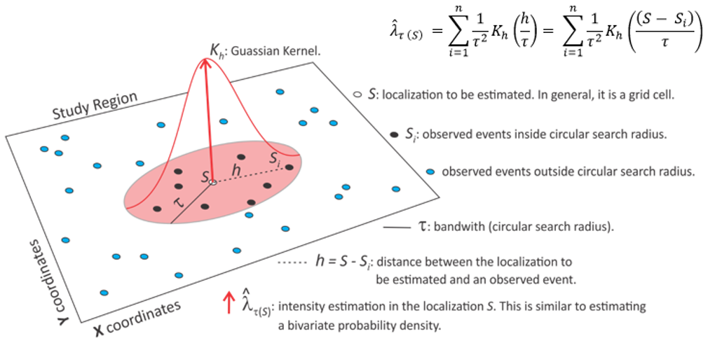
Normal (Gaussian): this function weights the observed points within the circular search
radius, so that the points closer to the location to be estimated are given
greater weight and vice versa.
Triangular: this function weights the observed points within
the circular search radius, so that the points closer to the location to be
estimated are given greater weight and vice versa, but the decrease is faster.
Uniform: this function assigns equal weights to all observed points that are within the circular search radius.
Negative Exponential: this function weights the observed points within
the circular search radius, so that the points closer to the location to be
estimated are given much greater weight than the most distant points.
Estimatation: estimates for the Kernel Map can be:
Density: calculates a surface
whose value will be proportional to the intensity of samples per unit area.
Spatial Moving Average: calculates the expected number of events per area unit.
Probability: calculates the probability of an events to be located in a given area.
Adaptive: it is a variable search radius. It is automatically calculated based on the geometry and the number of events on study area. In general, results of Kernel Maps created with adaptive radius are reasonably good.
Radius is an important parameter to create a Kernel map and
requires the user to understand the study region.
TerraView facilitates the definition task by allowing the creation of
Adaptive Kernel map. Adaptive option calculates a radius automatically
based on the number of events and the area.
However, Adaptive option can be unselected and the user can set the radius based on the width of the study
area. This value is set using percentage compared to the total width.
4. Output
Repository: defines where the
output PATH where the output layer will be saved and also its name. Press the button 
Layer Name: it shows the output layer name defined above.
Press the OK button to estimate the Kernel Map.
BIBLIOGRAPHIC REFERENCE
Bailey, Trevor C; Gatrell, Anthony C. Interactive spatial data analysis. Harlow Essex, England: Longman Scientific & Technical; New York, NY: J. Wiley, 1995.