At this point, a number of definitions and explanations of standard spatial statistical notations are required. A measure of spatial dependence is bound to make some assumptions about the underlying data generation process or processes. Among the assumptions that have been used in studies of autocorrelation, the one implying least about our prior knowledge of relationships between observations for spatial units, say point sites, or bounded zones exhaustively dividing up the study area, is based on contiguity. It is not usual to be able to estimate these relationships from data, involving as they do ![]() interactions, omitting those within zones; they are not the same as zonal fixed effects either, although the elimination of such fixed effects in panel studies can alter the ways in which interaction may appear.
interactions, omitting those within zones; they are not the same as zonal fixed effects either, although the elimination of such fixed effects in panel studies can alter the ways in which interaction may appear.
Cliff and Ord (1973, p. 11-13) provide the initial formalization of the relationships as a generalized weighting matrix, most usually termed ![]() . The most recent systematization, reviewing the Markovian properties of some weighting matrices is given by Bavaud (1998). In a recent study reviewing the use of different forms of weighting matrices, Griffith (1995) has demonstrated that a parsimonious specification of the relationships between observations is to be preferred to one making assumptions about say distance decay. Brett and Pinkse (1997) also note differences in inference which can occur in using distance bands and contiguities, which they call ``Hotelling neighbours'' for obvious reasons.
. The most recent systematization, reviewing the Markovian properties of some weighting matrices is given by Bavaud (1998). In a recent study reviewing the use of different forms of weighting matrices, Griffith (1995) has demonstrated that a parsimonious specification of the relationships between observations is to be preferred to one making assumptions about say distance decay. Brett and Pinkse (1997) also note differences in inference which can occur in using distance bands and contiguities, which they call ``Hotelling neighbours'' for obvious reasons.
It is usual in the literature to define the contiguity relation in terms of sets ![]() of neighbours of zone or site i. These are coded in the form of a weights matrix
of neighbours of zone or site i. These are coded in the form of a weights matrix ![]() , with a zero diagonal, and the off-diagonal non-zero elements often scaled to sum to unity in each row (a.k.a. standardized weights matrices), with typical elements:
, with a zero diagonal, and the off-diagonal non-zero elements often scaled to sum to unity in each row (a.k.a. standardized weights matrices), with typical elements:

where ![]() if i is linked to j and
if i is linked to j and ![]() otherwise. This implies no use of other information than that of neighbourhood set membership. Set membership may be defined on the basis of shared boundaries, of centroids lying within distance bands, or other a priori grounds.
otherwise. This implies no use of other information than that of neighbourhood set membership. Set membership may be defined on the basis of shared boundaries, of centroids lying within distance bands, or other a priori grounds.

Figure 1: Lattices of irregular polygon zones and point sites.
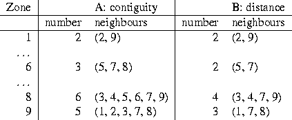
Figure 1A shows the way in which the sets of contiguous neighbours of each zone are constructed; in Figure 1B, neighbours are defined within a fixed distance from the zone in question. In table form, the sets of neighbours for selected zones are shown in Table 1.

Table 1: Neighbourhood sets for lattices shown in Figure 1.
As Getis and Ord point out (1992, p. 190), there are good reasons for examining patterns of spatial dependence at a more local scale. If we do not have good reason to suppose that the process in question is spatially stationary, it seems natural to apply distance-based tests to the observed spatial series. For use with distance statistics, one defines a symmetric one/zero spatial weighting matrix using the distance between the coordinates of a point associated with the observations. The choice of point for non-site series is not arbitrary, nor is the choice of the distance metric. Here the administrative centres of the observation units have been taken as adequately representing the location of the observation. Distance has been assumed to be the simple Euclidean distance between points, ignoring barriers and other factors. Distance has further been banded on the basis of the frequencies of interpoint distances, and the furthest nearest neighbour distance as shown in Figure 2. A typical element of the non-standardized spatial weight matrix ![]() for distance d is defined as:
for distance d is defined as:
![]()
and ![]() .
.
The extent to which results are affected by the choice of points representing zones, and the choice of a simple representation of distance is unknown. Distance banded spatial weight matrices may be stored in the same fashion as contiguity matrices, and may also be represented as sliced increments, again reducing storage requirements.

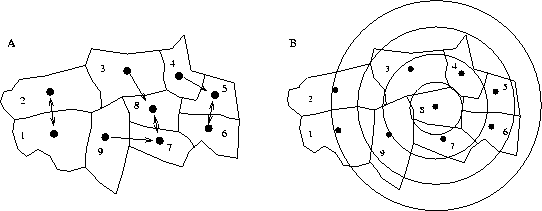
Figure 2: Nearest neighbours and distance bands.
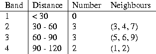
In Figure 2A, the nearest neighbours of each zone are shown. It is zone 9 that has the furthest nearest neighbour distance, at 50 km from zone 7, while zone 3 is 39 km from zone 8. Figure 2B illustrates the use of distance bands, at 30, 60, 90, and 120 km. Table 2 shows the incremental neighbourhood sets for zone 8 for these bands. If zones were permitted to be their own neighbours, then zone 8 would belong to the set of neighbours for band 1.

Table 2: The incremental neighbourhood sets of zone 8 (Figure 2B).

Table 3: Spatial lag values for zone 8.
We can exemplify the spatial lag using the neighbourhood set for zone 8 from Figure 1 and Table 1. If the set of observations from all the nine zones is (10.0, 12.0, 15.0, 17.0, 19.0, 18.0, 17.0, 16.0, 14.0), then we can see from Table 3 how the spatially lagged value is calculated as a sum or an average of the values of six neighbours of zone 8, in this case. The average lagged value of 16.67 corresponds closely to the observed value of 16.0.
Using these constructions, we can define two commonly used global measures of spatial autocorrelation (Cliff and Ord, 1973, p. 12, Haining, 1990, p. 230), Moran's I:

taking differences from the mean: ![]() , and the Geary coefficient:
, and the Geary coefficient:

In addition, mention should be made of the general class of cross product statistics due to Mantel (1967), and developed by Hubert et al. (1981):
![]()
If we set ![]() , we can express the Moran coefficient as
, we can express the Moran coefficient as ![]() , while the Geary measure takes the form:
, while the Geary measure takes the form: ![]() .
. ![]() yields a general framework for the development of additional measures, including space-time interaction and multivariate tests (Haining, 1990, p. 230-231).
yields a general framework for the development of additional measures, including space-time interaction and multivariate tests (Haining, 1990, p. 230-231).
The Moran and Geary coefficients may be tested using analytical expectations and variances (Cliff and Ord, 1973) based largely on the neighbourhood structure assumed in the spatial weighting matrix, and are asymptotically normally distributed. In addition to tests for interval scaled variables, there are also join-count statistics for nominal variables, based as the name suggests on counting the numbers of same-colour and different-colour joins between neighbours defined by the weighting scheme adopted. Lowell (1997) provides a review of these measures in the light of more recent developments. A study adapting Moran's I to heteroscedasticity has been conducted by Waldhör (1996), who is concerned with situations when testing the observed estimate of the statistic against a null in which any permutation of values to zones is not equally likely, an assumption underlying the analytical expectation and variance of the measure. Finally, new measures have been introduced by Sherman and Carlstein (1994) and Sherman (1996) using a method-of-moments solution using only the data at hand, and by Brett and Pinkse (1997) for spatial independence based on characteristic functions. The Moran statistic has been used in studies of prices in international trade by Aten (1996, 1997).